Theoretical model

The Kinetic Collective Model

The Kinetic Collective Model (KCM) developed in recent years improve the solution provided under the classical RTA. The model, derived from the exact solution of the LBTE proposed by Guyer and Krumhansl, is based on the splitting of the collision operator in normal and resistive processes (C = N + R ) when calculating the scattering matrix. As normal processes does not contribute directly to thermal resistance but redistribute momentum over all the phonon distribution, a suitable way to solve the LBTE is by using the basis that diagonalizes the normal scattering collision operator. This diagonalization allows to solve the BTE without complicating drastically the form of the drift operator.

The splitting of the collision operator allows to split the thermal conductivity in two contributions, kinetic and collective, weighed by a switching factor Σ :

κ = (1-Σ)κ^∗_K + Σκ^∗_C = κ_K + κ_C ,

where Σ=(1+$⟨$τ_N$⟩$ / $⟨$τ_R$⟩$)^-1. Σ ∈ [0,1] measures the relative importance of the N versus R phonon scattering. $⟨$τ$⟩$ represents a temperature dependent averaged relaxation time. While κ^∗ is the limit thermal conductivity in each regime, κ_K and ;&kappa_C are the actual contributions to thermal conductivity weighed by Σ. In the current version of KCM.py are implemented the contributions that maximizes the entropy in each regime as defined here:

κ^∗_K=∑_iC_iv_i⊗v_iτ_i

κ∗C=	∑iCiviqi⊗∑iCiviqi ∑iCiqi2/(ℏω)2τi-1

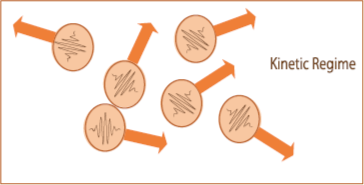
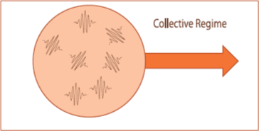
In the kinetic regime, each phonon behave independently, but in the collective regime, due to the effect of N collisions appears a coupling between phonons. Therefore phonons of different modes perform as a whole resistive collisions and share the same collision mean free time (MFT), the so-called collective MFT τ_c. In analogy with the definition of the thermal conductivity, the total phonon relaxation time can be defined from the kinetic or resistive MFT τ_K and the collective MFT τ_C as:

τ = (1-Σ)τ^∗_K + Στ^∗_C = τ_K + τ_C .

For a full understanding of the KCM look at REFERENCES.

Hydrodynamic heat transport in KCM

Since more than 10years ago the nanoTransport Group has been working in heat hydrodynamics and its applications to study nanoscale systems (see REFERENCES).

As pointed out previously, using the basis that diagonalizes the normal scattering collision operator allows to study the drift operator in a simple way to higher orders, leading to an hydrodynamic equation beyond Fourier:

∂τ/∂t + q = -κ∇T+ℓ²(∇²q+2∇∇q) ,

where $\ell$ is the non-local length (NL-param). From Guyer and Krumhansl it is studied the limiting case where normal proceses dominate, τ_N«τ_R. In this limit, corresponding to the collective regime, the NL-param is $\ell 2$_C^∗=⟨v²τ_N⟩⟨τ_C⟩.

To have a global equation, in the KCM framework has been studied the kinetic limit τ_N»τ_R, leading to $\ell 2$_K^∗=⟨v²τ_R⟩⟨τ_R⟩. This generalization allows to define a total non-local length as:

ℓ² = (1-Σ)ℓ²_K^∗ + Σℓ²_C^∗ = ℓ²_K + ℓ²_C .

This extension of the Guyer and Krumhansl equation done in the KCM framework leads to the so-called hydrodynamic KCM equation (Eq.5). This equation, together with suitable boundary conditions, can be implemented for finite elements simulations to study thermal properties in complex geometries (see FINITE ELEMENTS).